UMN UAV Simulation: Linearize Tutorial
This tutorial walks through the steps of linearizing the UMN UAV Simulation model. Most of these steps are handled in the "setup.m" and "linearize_UAV.m" functions provided with the UMN UAV sim. However, this tutorial will give you an in-depth understanding of how these functions work.
Contents
Author: Austin Murch
University of Minnesota
Aerospace Engineering and Mechanics
Copyright 2011 Regents of the University of Minnesota.
All rights reserved.
SVN Info: $Id: linearize_tutorial.m 305 2011-03-16 16:17:53Z murch $
Setup and Configuration
Before we get started we need to make sure the MATLAB path is correct and we have all of the aircraft and simulation parameters are defined. This step is handled in setup.m.
% Add Libraries folder to MATLAB path
addpath ../Libraries
warning('off','Simulink:SL_LoadMdlParameterizedLink')

% Configure Airframe, either 'Ultrastick' or 'FASER'
[AC,Env] = UAV_config('Ultrastick');

% Simulation sample time
SampleTime = 0.02; % sec

% Load model into system memory without opening diagram
load_system('UAV_NL.mdl')
Aircraft configuration saved as: UAV_modelconfig.mat
Set Aircraft Initial Conditions and Trim the Model
Next we need to define initial conditions for the simulation model inputs and state vector and trim the model to a particular flight condition. This step is handled in setup.m.
% Set the initial model inputs
TrimCondition.Inputs.elevator = 0.091; % rad
TrimCondition.Inputs.aileron  = 0;     % rad
TrimCondition.Inputs.rudder   = 0;     % rad
TrimCondition.Inputs.flap     = 0;     % rad
TrimCondition.Inputs.throttle = 0.559; % nd, 0 to 1

% Set initial state values
TrimCondition.InertialIni    = [0 0 -100]';   % Initial Position in Inertial Frame [Xe Ye Ze], [m]
TrimCondition.LLIni          = [45 -122];     % Initial Latitude/Longitude of Aircraft [Lat Long], [deg]
TrimCondition.VelocitiesIni  = [17 0 0.369]'; % Initial Body Frame velocities [u v w], [m/s]
TrimCondition.AttitudeIni    = [0 0.0217 0]'; % Initial Euler orientation [roll,pitch,yaw] [rad]
TrimCondition.RatesIni       = [0 0 0]';      % Initial Body Frame rotation rates [p q r], [rad/s]
TrimCondition.EngineSpeedIni = 827;           % Initial Engine Speed [rad/s]

% Set the trim target
TrimCondition.target = struct('V_s',17,'gamma',0); % straight and level, (m/s, rad)

% Find the trim solution
[TrimCondition,OperatingPoint] = trim_UAV(TrimCondition,AC);
Local minimum found that satisfies the constraints.

Optimization completed because the objective function is non-decreasing in
feasible directions, to within the default value of the function tolerance,
and constraints were satisfied to within the default value of the constraint tolerance.


No active inequalities.

 Operating Point Search Report:
---------------------------------

 Operating Report for the Model UAV_NL.
 (Time-Varying Components Evaluated at time t=0)

Operating point specifications were successfully met.

States:
----------
(1.) UAV_NL/Nonlinear UAV Model/6DoF EOM/Calculate DCM & Euler Angles/phi theta psi
      x:       -0.0015      dx:      1.9e-024 (0)
      x:        0.0522      dx:      4.5e-023 (0)
      x:             0      dx:      2.1e-023 (0)
(2.) UAV_NL/Nonlinear UAV Model/6DoF EOM/p,q,r
      x:     8.05e-025      dx:     4.96e-012 (0)
      x:      4.5e-023      dx:    -9.15e-015 (0)
      x:      2.1e-023      dx:     3.77e-013 (0)
(3.) UAV_NL/Nonlinear UAV Model/6DoF EOM/ub,vb,wb
      x:            17      dx:     7.65e-012 (0)
      x:     2.42e-021      dx:     1.15e-016 (0)
      x:         0.887      dx:     9.35e-015 (0)
(4.) UAV_NL/Nonlinear UAV Model/Auxiliary Equations/xe,ye,ze
      x:      7.1e-015      dx:            17
      x:     2.46e-014      dx:       0.00133
      x:          -100      dx:    -1.44e-015
(5.) UAV_NL/Nonlinear UAV Model/Forces and Moments/Electric Propulsion Forces and Moments/Engine speed Integrator
      x:           826      dx:     1.43e-009 (0)

Inputs:
----------
(1.) UAV_NL/elevator
      u:       -0.0772    [-0.436 0.436]
(2.) UAV_NL/aileron
      u:       0.00993    [-0.436 0.436]
(3.) UAV_NL/rudder
      u:       0.00269    [-0.436 0.436]
(4.) UAV_NL/throttle
      u:         0.568    [0 1]
(5.) UAV_NL/flap
      u:             0

Outputs:
----------
(1.) UAV_NL/V_s
      y:            17    (17)
(2.) UAV_NL/beta
      y:     1.43e-022    (0)
(3.) UAV_NL/alpha
      y:        0.0522    [-Inf Inf]
(4.) UAV_NL/h
      y:          79.1    [-Inf Inf]
(5.) UAV_NL/phi
      y:       -0.0015    [-Inf Inf]
(6.) UAV_NL/theta
      y:        0.0522    [-Inf Inf]
(7.) UAV_NL/psi
      y:             0    [-Inf Inf]
(8.) UAV_NL/p
      y:     8.05e-025    [-Inf Inf]
(9.) UAV_NL/q
      y:      4.5e-023    [-Inf Inf]
(10.) UAV_NL/r
      y:      2.1e-023    [-Inf Inf]
(11.) UAV_NL/gamma
      y:    -8.49e-017    (0)


 Trim conditions saved as:	 UAV_trimcondition.mat
Linearize the Model
Linearizing is done using the "linearize.m" built-in function. We need to pass this function the model name and an operating point object that we get from trim_UAV. A linear model is only relevant when created around a trimmed flight condition.
linmodel = linearize('UAV_NL',OperatingPoint.op_point);
Full Linear Model
We now have a full 13-state linear model, but the state, input, and output names need to be made consistent. Note the "\" in the name will format the name as a greek symbol when plotting.
set(linmodel, 'InputName', {'\delta_e' ;'\delta_a'; '\delta_r';'\delta_t';'\delta_f'});
set(linmodel, 'OutputName',{'V'; '\beta'; '\alpha'; 'h'; '\phi'; '\theta';'\psi';'p';'q';'r';'gamma'});
set(linmodel, 'StateName', {'\phi';'\theta';'\psi';'p';'q';'r';'u';'v';'w';'Xe';'Ye';'Ze';'\omega'})
linmodel
a =
                  \phi       \theta         \psi            p            q
   \phi     2.352e-024   2.101e-023            0            1  -7.846e-005
   \theta  -2.095e-023            0            0            0            1
   \psi     4.509e-023   1.096e-024            0            0    -0.001504
   p                 0            0            0       -13.08      -0.1051
   q                 0            0            0  -1.135e-021       -9.396
   r                 0            0            0       0.3732      -0.6711
   u                 0       -9.793            0            0      -0.8424
   v             9.793    0.0007684            0       0.8468            0
   w           0.01471      -0.5116            0  -2.423e-021        15.68
   Xe       6.949e-005   4.693e-012    -0.001332            0            0
   Ye          -0.8869            0           17            0            0
   Ze          0.00133          -17            0            0            0
   \omega            0            0            0            0            0

                     r            u            v            w           Xe
   \phi        0.05224            0            0            0            0
   \theta     0.001502            0            0            0            0
   \psi          1.001            0            0            0            0
   p             3.005      -0.1475       -2.406     -0.01411   3.876e-010
   q            0.7427        0.209     -0.04514       -4.001   2.819e-024
   r            -2.566     -0.01064        1.532     -0.04146    3.35e-011
   u        2.423e-021      -0.6134    -0.000864       0.8094  -5.825e-010
   v            -16.82     0.001728      -0.9007   9.027e-005  -1.675e-011
   w                 0      -0.7457  -4.514e-005       -7.808   1.115e-008
   Xe                0       0.9986  -7.836e-005      0.05217            0
   Ye                0            0            1     0.001502            0
   Ze                0     -0.05217      -0.0015       0.9986            0
   \omega            0        135.7   1.937e-020        7.091   2.632e-007

                    Ye           Ze       \omega
   \phi              0            0            0
   \theta            0            0            0
   \psi              0            0            0
   p        1.336e-009    -0.000121    -0.001524
   q        9.716e-024    -8.8e-019   1.891e-026
   r        1.155e-010  -1.046e-005   -0.0001317
   u       -5.432e-010   4.904e-005      0.01298
   v       -1.562e-011    1.41e-006            0
   w         1.04e-008   -0.0009387            0
   Xe                0            0            0
   Ye                0            0            0
   Ze                0            0            0
   \omega    9.07e-007     -0.08215       -5.903

b =
              \delta_e     \delta_a     \delta_r     \delta_t     \delta_f
   \phi              0            0            0            0            0
   \theta            0            0            0            0            0
   \psi              0            0            0            0            0
   p                 0       -127.8        4.195        3.683            0
   q            -79.95  -1.123e-020   7.844e-022            0        4.399
   r                 0        9.739       -76.52       0.3183            0
   u            0.4825      -0.8636      -0.8664            0       0.7259
   v                 0            0        5.478            0            0
   w            -2.793     -0.04511     -0.04526            0       -21.18
   Xe                0            0            0            0            0
   Ye                0            0            0            0            0
   Ze                0            0            0            0            0
   \omega            0            0            0         2500            0

c =
                  \phi       \theta         \psi            p            q
   V                 0            0            0            0            0
   \beta             0            0            0            0            0
   \alpha            0            0            0            0            0
   h                 0            0            0            0            0
   \phi              1            0            0            0            0
   \theta            0            1            0            0            0
   \psi              0            0  -3.142e+005            0            0
   p                 0            0            0            1            0
   q                 0            0            0            0            1
   r                 0            0            0            0            0
   gamma    7.825e-005           -1   9.067e-031            0            0

                     r            u            v            w           Xe
   V                 0       0.9986   1.425e-022      0.05217            0
   \beta             0  -8.373e-024      0.05882  -4.374e-025            0
   \alpha            0    -0.003069            0      0.05874            0
   h                 0            0            0            0   3.203e-006
   \phi              0            0            0            0            0
   \theta            0            0            0            0            0
   \psi              0            0            0            0            0
   p                 0            0            0            0            0
   q                 0            0            0            0            0
   r                 1            0            0            0            0
   gamma             0    -0.003069  -8.823e-005      0.05874            0

                    Ye           Ze       \omega
   V                 0            0            0
   \beta             0            0            0
   \alpha            0            0            0
   h        1.104e-005           -1            0
   \phi              0            0            0
   \theta            0            0            0
   \psi              0            0            0
   p                 0            0            0
   q                 0            0            0
   r                 0            0            0
   gamma             0            0            0

d =
           \delta_e  \delta_a  \delta_r  \delta_t  \delta_f
   V              0         0         0         0         0
   \beta          0         0         0         0         0
   \alpha         0         0         0         0         0
   h              0         0         0         0         0
   \phi           0         0         0         0         0
   \theta         0         0         0         0         0
   \psi           0         0         0         0         0
   p              0         0         0         0         0
   q              0         0         0         0         0
   r              0         0         0         0         0
   gamma          0         0         0         0         0

Continuous-time model.
From the full model we can generate transfer functions between the inputs and the relevant outputs. These are stored in the "TF" data structure.
% Generate transfer functions from statespace data
TF.full_elev2q = tf(linmodel(9,1));% elev to output 9 (q)
TF.full_ail2p  = tf(linmodel(8,2));% ail to output 8 (p)
TF.full_ail2r  = tf(linmodel(10,2));% ail to output 10 (r)
TF.full_rud2p  = tf(linmodel(8,3));% rud to output 8 (p)
TF.full_rud2r  = tf(linmodel(10,3));% rud to output 10 (r)
Reduced Order Longitudinal Model
The full 13 state linear model is a bit cumbersome to work with, so we normally separate the model into two decoupled, reduced order models: one for the longitudinal axis and another for the lateral-directional axes.
The longitudinal model has 5 states: forward velocity, vertical velocity, pitch rate, pitch angle, vertical position, and motor speed (u, w, q, \theta, Ze, \omega). 2 inputs: elevator and throttle, (\delta_e, \delta_t). and 5 outputs: airspeed, angle of attack, pitch rate, pitch angle, and altitude. (V_s, \alpha, q, \theta, h). We can reduce the full linear model using model reduction with the "modred" function. We first define indices corresponding to the states, outputs, and inputs we wish to retain in the linear model. We then need to reorder the state vector to the order listed above.
% Generate State-space matrices for Longitudinal Model
% Indices for desired state, outputs, and inputs that we want to keep
Xlon = [7 9 5 2 12 13];
Ylon = [1 3 9 6 4];
Ilon = [1 4];
longmod = modred(linmodel(Ylon,Ilon),setdiff(1:13,Xlon),'Truncate');

% Reorder state vector
longmod = xperm(longmod,[3 4 1 2 5 6])
a =
                    u           w      \theta           q          Ze      \omega
   u          -0.6134      0.8094      -9.793     -0.8424  4.904e-005     0.01298
   w          -0.7457      -7.808     -0.5116       15.68  -0.0009387           0
   \theta           0           0           0           1           0           0
   q            0.209      -4.001           0      -9.396   -8.8e-019  1.891e-026
   Ze        -0.05217      0.9986         -17           0           0           0
   \omega       135.7       7.091           0           0    -0.08215      -5.903

b =
           \delta_e  \delta_t
   u         0.4825         0
   w         -2.793         0
   \theta         0         0
   q         -79.95         0
   Ze             0         0
   \omega         0      2500

c =
                   u          w     \theta          q         Ze     \omega
   V          0.9986    0.05217          0          0          0          0
   \alpha  -0.003069    0.05874          0          0          0          0
   q               0          0          0          1          0          0
   \theta          0          0          1          0          0          0
   h               0          0          0          0         -1          0

d =
           \delta_e  \delta_t
   V              0         0
   \alpha         0         0
   q              0         0
   \theta         0         0
   h              0         0

Continuous-time model.
Now we have a reduced order linear model for the longitudinal dynamics. From this linear model we can generate transfer functions between the inputs and the relevant outputs. These are stored in the "TF" data structure.
% Generate transfer functions from statespace data
% TFs from elevator to outputs
TF.elev2Vs    = tf(longmod(1,1));% elev to output 1 (V)
TF.elev2alpha = tf(longmod(2,1));% elev to output 2 (alpha)
TF.elev2q     = tf(longmod(3,1));% elev to output 3 (q)
TF.elev2theta = tf(longmod(4,1));% elev to output 4 (theta)
TF.elev2h     = tf(longmod(5,1));% elev to output 5 (h)

% TFs from throttle to outputs
TF.thr2Vs    = tf(longmod(1,2));% thr to output 1 (V)
TF.thr2alpha = tf(longmod(2,2));% thr to output 2 (alpha)
TF.thr2q     = tf(longmod(3,2));% thr to output 3 (q)
TF.thr2theta = tf(longmod(4,2));% thr to output 4 (theta)
TF.thr2h     = tf(longmod(5,2));% thr to output 5 (h)
Reduced Order Lateral-Directional Model
The lateral-directional model has 5 states: side velocity, roll rate, yaw rate, roll angle, and yaw angle . (v, p, r, \phi, \psi). 2 inputs: aileron and rudder, (\delta_a, \delta_r). and 5 outputs: sideslip angle, roll rate, yaw rate, roll angle, and yaw angle (\beta, p, r, \phi, \psi). We can reduce the full linear model using model reduction with the "modred" function. We first define indices corresponding to the states, outputs, and inputs we wish to retain in the linear model. We then need to reorder the state vector to the order listed above.
% Generate State-space matrices for lateral-directional Model
% Indices for desired state, outputs, and inputs that we want to keep
Xlat = [8 4 6 1 3];
Ylat = [2 8 10 5 7];
Ilat = [2 3];
latmod = modred(linmodel(Ylat,Ilat),setdiff(1:13,Xlat),'Truncate');
latmod = xperm(latmod,[5 3 4 1 2]); % reorder state
Now we have a reduced order linear model for the lateral-directional dynamics. From this linear model we can generate transfer functions between the inputs and the relevant outputs. These are stored in the "TF" data structure.
% Generate transfer functions from statespace data
% TFs from aileron to outputs
TF.ail2v   = tf(latmod(1,1));% ail to output 1 (v)
TF.ail2p   = tf(latmod(2,1));% ail to output 2 (p)
TF.ail2r   = tf(latmod(3,1));% ail to output 3 (r)
TF.ail2phi = tf(latmod(4,1));% ail to output 4 (phi)
TF.ail2psi = tf(latmod(5,1));% ail to output 5 (psi)

% TFs from rud to outputs
TF.rud2v   = tf(latmod(1,2));% rud to output 1 (v)
TF.rud2p   = tf(latmod(2,2));% rud to output 2 (p)
TF.rud2r   = tf(latmod(3,2));% rud to output 3 (r)
TF.rud2phi = tf(latmod(4,2));% rud to output 4 (phi)
TF.rud2psi = tf(latmod(5,2));% rud to output 5 (psi)
Longitudinal Model Analysis
Now that we have linear models, let's look at the bode plot of a few relevant cases: first we'll look at elevator to pitch rate, comparing the full model to the reduced order model.
figure
bode(TF.full_elev2q,TF.elev2q,{.01,1000}); grid on
legend('Full Model','Reduced Order Model')
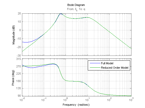
We see that there is very little difference between the two models for any reasonable frequencies, so the reduced order model is a good approximation. We can also see the two dominant modes of the system, the Phugoid and short period, in the two humps in the magnitude plot. Also of interest is where the magnitude crosses zero- this defines the bandwidth of the system response.
The best way to look at the modes of the system is to look at the Eigenvalues; for this, we'll use the "damp" function.
damp(longmod)
        Eigenvalue            Damping     Freq. (rad/s)

 -1.57e-004                  1.00e+000      1.57e-004
 -1.55e-001 + 5.36e-001i     2.77e-001      5.58e-001
 -1.55e-001 - 5.36e-001i     2.77e-001      5.58e-001
 -6.22e+000                  1.00e+000      6.22e+000
 -8.60e+000 + 7.90e+000i     7.36e-001      1.17e+001
 -8.60e+000 - 7.90e+000i     7.36e-001      1.17e+001
This shows us the Eigenvalues of the system, as well as their frequency and damping. We see the Phugoid mode, with reasonable damping and normal low frequency. The Short Period mode is the other complex pair, with a good damping ratio and reasonable frequency.
Lateral-Directional Model Analysis
For the lateral-directional model, let's look at aileron to roll rate and rudder to yaw rate.
figure
bode(TF.full_ail2p,TF.ail2p,{.01,1000}); grid on
legend('Full Model','Reduced Order Model')
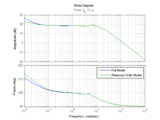
Again, we see that there is very little difference between the two models for any reasonable frequencies, so the reduced order model is a good approximation. We can also see the dominant behavior of the roll axis, in that the roll rate response behaves as a first-order system.
Now the rudder to yaw rate:
figure
bode(TF.full_rud2r,TF.rud2r,{.01,1000}); grid on
legend('Full Model','Reduced Order Model')
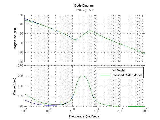
Again, the reduced order model is a good approximation. The hump in the magnitude is the Dutch Roll mode.
The best way to look at the modes of the system is to look at the Eigenvalues; for this, we'll use the "damp" function.
damp(latmod)
        Eigenvalue            Damping     Freq. (rad/s)

  0.00e+000                 -1.00e+000      0.00e+000
 -1.49e-002                  1.00e+000      1.49e-002
 -1.74e+000 + 5.06e+000i     3.25e-001      5.35e+000
 -1.74e+000 - 5.06e+000i     3.25e-001      5.35e+000
 -1.31e+001                  1.00e+000      1.31e+001
This shows us the Eigenvalues of the system, as well as their frequency and damping. We see the Dutch Roll mode is the only complex pair of Eigenvalues, with a lower damping ratio and moderate frequency. The roll mode is first order and relatively fast; the slow first order mode is the spiral mode, which can be unstable for some aircraft.
This concludes the linearize tutorial. Please send any comments or questions to Austin Murch (murch@aem.umn.edu).